Beyond the glitter
Despite its reputation, gold has a poor record as an investment. That doesn’t mean it’s not a good trading vehicle, though.
Gold is often referred to as a safe-haven for investors during times of economic uncertainty. Unfortunately iq option cheat or not?, while for many investors and traders there have been plenty of financial calamities that would justify moving assets into gold, the yellow metal is not the safe haven it once was. Gold traded above $850.00 an ounce in 1980 (Figure 1), a price investors and traders have not seen since. Following this peak, however, gold was essentially in a bear market until 2002, when the market successfully tested support around $250. Then, in concert with global economic expansion, demand for gold pushed the price temporarily over $700 an ounce in 2006. For the past year (June 2006 through May 2007), gold has been in a broad trading range, from just below $600 to just over $700 an ounce.
Despite its unfavorable performance as a long-term investment, gold is nonetheless a market that presents opportunities for nimble traders. Here, we explore the short-term trading characteristics of this market to see how best to trade it day to day.
Traders can buy and sell gold nearly 24 hours a day. Gold futures are traded on two exchanges — the New York Mercantile Exchange (NYMEX), which has pit- and electronically traded contracts, and the Chicago Board of Trade (CBOT), which has an electronically-traded mini gold contract. The following analysis reviews daily data for the CBOT mini gold futures (ticker symbol: YG) from June 1, 2006 through May 31, 2007, a total of 251 trading days. The study determines key market statistics for short-term traders, including daily range, close-to-close changes, how low the market tends to trade down on days it closes higher, and how high it tends to trade on days it closes lower. Intraday analysis of hourly price data from April 2007 through May 31, 2007 is also included. The electronic NYMEX gold price data is used to identify times of the day when gold offers the most price action. Figure 2 is a daily continuous futures gold chart from June 1, 2006 through May 31, 2007. Gold hit its low during the review period during the middle of June (after peaking the month before) and then rallied to form its high for the review period in July. Since that broad swing, gold has been moving sideways, with the market spending the final quarter of the review period in the upper half of its year-long range. Let’s see what this market tends to do from day to day.
Daily bar characteristics
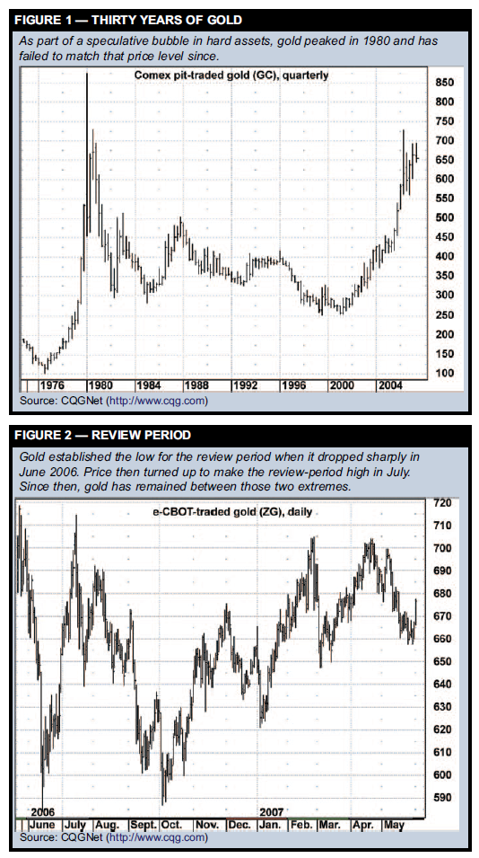
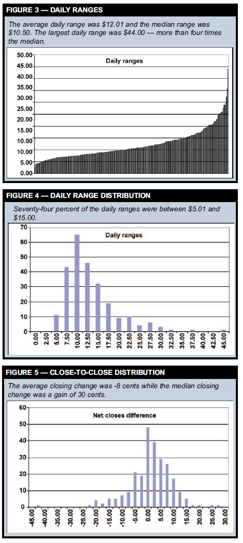
Figure 3 shows the daily ranges for the review period sorted from smallest to largest. The smallest range ($2.80) occurred on Dec. 26, 2006 and the largest ($44.00) occurred on June 13, 2006 — one day ahead of the bottom. The average daily range was $12.01 and the median range was just $10.50. The difference between the average and the median indicates outliers — several large-range days evident on the right side of the chart — pushed the average range figure higher. In this case, the median range is more indicative of the “typical” behavior one would expect in this market. Figure 4 is a frequency distribution chart of the daily ranges. Frequency distribution analysis measures the number of times the daily ranges fell within a certain range. In this case, the horizontal axis is the daily range in increments of $2.50 from left to right with each value displayed representing the upper limit of the range for the respective category. For example, the daily range was greater than $7.50 up to and including $10.00 over 60 times (the value on the Y axis). We can see the one outlier where the $44.00 daily range fell into the last category. Seventy-four percent of the daily ranges were greater than $5.00 and up to and including $15.00. The daily range exceeded $25.00 only 5 percent of the time (12 sessions). Analyzing the close-to-close behavior shows that the largest one-day net loss on a closing basis was -$43.90 on June 13, 2006, and the largest one-day closing gain was $26.90 on June 30, 2006. The market never closed without either a gain or a loss for the session. Figure 5 shows the frequency distribution for close-to-close differences. The peak number of closing differences fell in the range of a loss of more than -$2.50 up to unchanged. The average close-to-close change was a loss of $0.08 and the median was a gain of $0.30. Eighty-four percent of the close-to-close differences were between a loss of $10.00 and a gain of $10.00. The close-to-close changes exceeded $10.00 to the upside 7 percent of the time and the close-to-close changes were losses greater than – $10.00 seven percent of the time. The market closed up 51 percent of the time. Figure 6 displays a chart of the daily bars when the close was greater than the previous day’s close. The bars are adjusted so that the previous day’s close is the zero line, and the individual bar’s range is relative to the zero line. The market closed in positive territory 129 days. We can see the effect of volatility working its way lower over the review period. The left-hand side of the chart shows daily lows more than -$10.00 below the previous day’s close, while the right-hand side of the chart shows the low was more than -$5.00 only five times.
Gold trading tendencies
Insights from the June 1, 2006 through May 31, 2007 review of gold price:
1. The average range was $12.01 and the median range was $10.50; 74 percent were between $5.01 and $15.00. The daily range exceeded $25.00 only 5 percent of the time (12 days).
2. The average close-to-close change was -$0.08, while the median close-to-close change was +$0.30 — a reminder of this market’s choppy nature. Eighty-four percent of the close-to-close differences ranged from a decline of $10.00 to a gain of $10.00. The close-to-close changes exceeded $10.00 to the upside seven percent of the time and exceeded -$10.00 to the downside seven percent of the time.
3. On up-closing days, the low was above the previous day’s close 22 percent of the time. The market traded down by $6 or more and still closed up on the day only 16 percent of the time.
4. On down-closing days, gold was up on the day 85 percent of the time (i.e., it failed to trade in positive territory only 15 percent of the time). After being more than up $5.00 on the day, gold closed down only 14 percent of the time.
5. Intraday analysis from April 1, 2007 through May 31, 2007 shows the 7:20 a.m. hour (which corresponds to the opening of the pit session for NYMEX gold) had the highest average range of 60-minute bars.
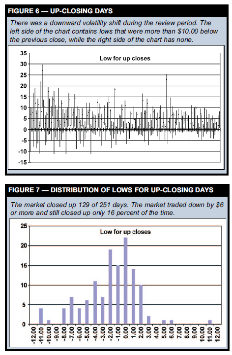
Figure 7 is a frequency distribution of the difference between the low and the previous day’s close for those sessions the market closed in positive territory. Twenty-nine or 22 percent of the time the low was above the previous day’s close. The largest positive difference between the low and the previous day’s close (a gap up opening) was $10.30 and the largest negative difference was – $11.30.
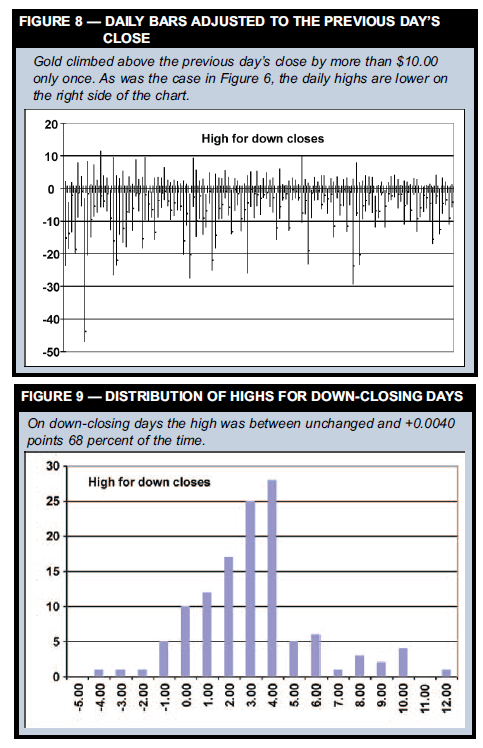
Seventy-eight percent of the time for those days the session closed up the low was between unchanged and down to a loss of $11.30. However, only 16 percent of the time did the low drop to $6.00 or more below the previous day’s close and the market recovered to close up for the session. Figure 8 is a chart of the sessions where the market closed down. Similar to Figure 5, the bars’ ranges and closing prices are adjusted relative to the previous day’s close. The high was only $10.00 ($11.40) above the previous close once for down closing sessions. Figure 9 is a frequency distribution of the highs for those sessions the market closed in negative territory. The market closed down 122 times during the review period. Eighteen sessions or 15 percent of the time the market did not trade in positive territory; therefore 85 percent of the time the market was up on the day for down closes. The largest difference between the high and the close for a gap down session was $4.30. Gold traded more than $5.00 above the previous day’s close and still closed down for the session only 14 percent of the time (17 sessions).
Intraday price action
The intraday analysis is based on 60-minute bars and a 24- hour clock (Central Time). The NYMEX pit-trading session opens at 7:20 a.m. and closes at 12:30 p.m. To account for both the electronic and pit-traded gold sessions, some changes are made to the data. The electronically traded gold data starts at 0:00 (midnight) and progresses in hourly increments. However, the 7 a.m. hour closes at 7:19:59 — just as the pit-session begins. Then, the 60- minute bars re-start at 7:20 to correspond to the pit session. Accordingly, the 7 a.m. “hour” is only 20 minutes long. Also, because the pit session closes at 12:30 p.m., the 12:20 “hour” is only 10 minutes long, with 60- minute increments beginning again at 12:30 p.m. At 4:15 p.m., the electronic trading session closes for 45 minutes, so the 3:30 p.m. hour is only 45 minutes long and the intraday analysis starts with the reopening of electronic trading at 5:00. By analyzing the 60-minute bars, we hope to identify the time of day when the market is the most volatile. The range for each 60-minute bar was calculated and sorted by hour (0:00 to 23:00). Next, both the average and the median were calculated for each period.
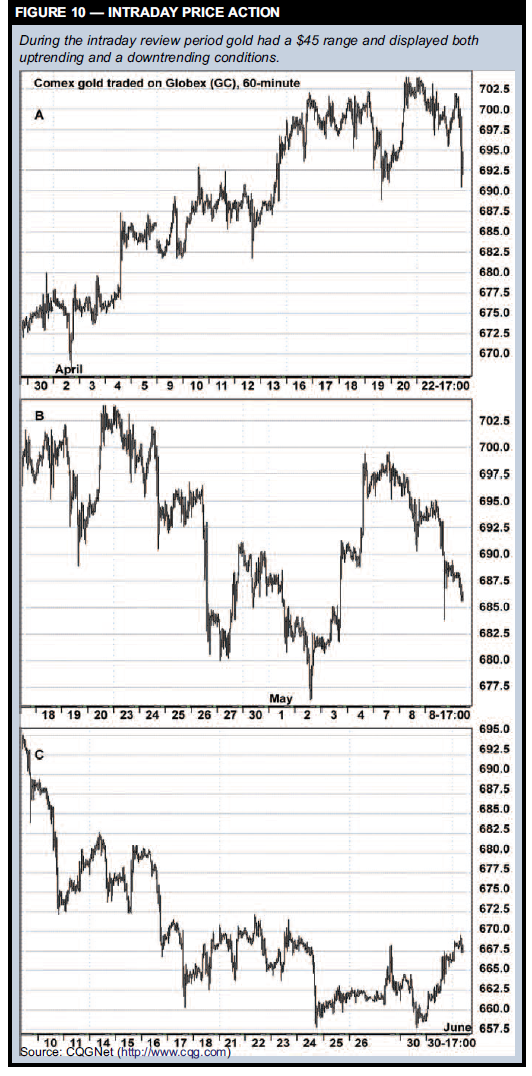
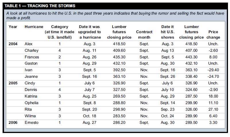
Figure 11 shows the average and median ranges for the different hours of the 24-hour trading day. Overall, the first three hours following the opening of the pit session at 7:20 a.m. were the most volatile. The 7:20 hour had the widest average range and the second-highest median range. The 9:20 hour had the biggest median range and the second-largest average range. The 8:20 hour came in third on both counts. The average for the 7:20 hour was $3.50 and the median was $3.00, a difference of $0.65. This relatively large difference suggests several largerange bars pushed up the average for this hour. The average and median values for the 9:20 hour were much closer, indicating the ranges for this hour were more consistent.
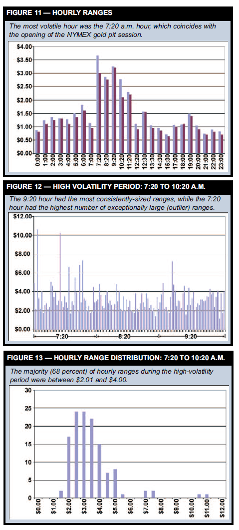
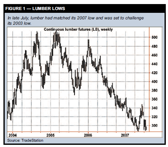
Figure 12, which shows the individ-ual ranges for the 7:20, 8:20, and 9:20 hours, highlights some of these observations. The range was $5.00 or more seven times in the 7:20 hour; the 9:20 hour had one range exceeding this threshold, and the 8:20 hour had none. Figure 13 shows the distribution of hourly ranges during the three highly volatile hours. Sixty-eight percent of the hourly ranges were greater than $2.00 up to and including $4.00; the hourly range was less than $2.00 only 15 percent of the time. The largest hourly reading was $10.60.
Keeping current
“Gold trading tendencies” (p. 10) summarizes some of the highlights of this analysis. Traders should remember that one of primary benefits of this type of research is staying abreast of changing market conditions that will affect the performance of trade strategies; as a result, such studies should be updated regularly — at least on a quarterly basis. Overall, gold has been a poor investment for many years, and there’s no telling how long the current bull market (which is already showing signs of fatigue) will persist. However, traders can take advantage of this market’s volatility by understanding its day-to-day behavior and structuring trade plans accordingly
The other weather market
Weather conditions during the upcoming hurricane season could have traders thinking twice about falling lumber prices (Figure 1). Weather affecting the markets is nothing new; commodity futures traders know weather markets can produce exciting trade opportunities, as increased market volatility and heightened investor interest spur major moves. Grains, orange juice, and heating oil are the best-known markets in which weather conditions can play a key role in prices. However, such opportunities also present themselves in lumber futures (LB), especially as the Atlantic hurricane season begins. According to the National Oceanic & Atmospheric Administration (http://www.noaa.gov), the season officially begins June 1 and runs through the end of November. More than 97 percent of tropical disturbances fall within this window, with peak activity usually between August and October. So how do traders react when weather forecasts predict tropical storms or hurricanes in the U.S.? Let’s take a look at three tropical storms that reached the U.S. over the past three years in August and early September — the heart of hurricane season — and what occurred in the lumber futures market just before, during, and after the storms went ashore in the U.S.
The Atlantic hurricane season officially begins June 1 and runs through the end of November. More than 97 percent of tropical disturbances fall within this window.
2004 Hurricanes are ranked from 1 to 5, with 5 being the strongest. In 2004, Hurricane Charley was a category 4 hurricane — the strongest storm to strike the U.S. in 12 years, causing serious damage to parts of the Florida peninsula. The storm first caught the attention of traders on Aug. 10, when a tropical depression in the southeastern Caribbean Sea strengthened to become Tropical Storm Charley. However, the lumber market showed no concerns, and prices fell sharply in the front-month September contract, as technical traders liquidated positions fearing a potential double-top formation on the daily chart (Figure 2). Charley continued to strengthen,
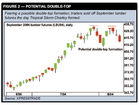
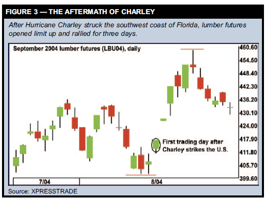
becoming a hurricane on Aug. 11 as the storm’s eye hovered just outside Jamaica. Lumber traders, however, continued their selling spree for the fourth consecutive session, causing prices to move to a one-month low. With the weekend approaching, Charley strengthened to a category 2 storm as it approached the Cayman Islands and Cuba, but the lumber market closed lower for a fifth consecutive session, reaching lows of $401.50 before a moderate short-covering rally cut the day’s decline. On Friday, Aug. 13, another shortcovering rally ensued, as weather forecasters were calling for Charley to move toward the southwest coast of Florida. Trading was choppy, but the failure to make new lows at $401.50 allowed prices to end the day with a modest gain of $3.50. Over the weekend Charley became a category 4 storm, with winds approaching 125 knots. It made landfall on the southwest coast of Florida and caused severe damage to the cities of Punta Gorda and Port Charlotte. Charley continued to maintain hurricane- strength winds as it moved inland, passing close to the Orlando area before moving back into the Atlantic just outside Daytona Beach. When trading resumed on Monday, Aug. 16, the news reports of the destruction caused by Charley sent a flurry of buy orders to the lumber pit, causing a gap opening and eventually sending prices up the $10 daily limit (Figure 3). On Tuesday, Aug. 17, only a small number of sell orders kept prices from opening limit bid. Once these orders were absorbed, the market once again closed limit-up. Wednesday was a wild day of trading, with price limits expanding to $15 and both bulls and bears fighting for control of the market. The bulls prevailed, and after posting a $13.50 daily range, September lumber closed up the expanded $15 limit. The poststorm rally continued for three more sessions, finally topping out at $458.70 on Aug. 23.
2005
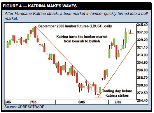
On Aug. 24, 2005, the 11th tropical storm of the 2005 season was officially named Katrina as it gained strength over the central Bahamas. The following day, Katrina gained hurricane status as its core moved over southeastern Florida. On this day, September lumber closed below the lower end of a nearly two-week trading range, as traders continued to focus on overproduction and large imports rather than potential storm threats. On Friday, Aug. 26, September lumber made its contract lows of $267. Traders finally started to take notice of the storm, and a short-covering rally ensued, sending September lumber up $8 to end the week. Over the weekend, Katrina strengthened to a category 5 storm as it headed for the Gulf coast. Early Monday morning, Katrina weakened to a strong category 3 storm as it reached land near Buras, La. Lumber futures opened that morning up the $10 limit and traded briefly off the limit before locking up the limit bid. Tuesday, prices opened sharply higher but did not touch the $10 limit, causing a selloff by weak longs that allowed the September contract to close the session with a small loss. That was the last chance for traders to enter the market on the long side or cover short positions before prices moved sharply higher. Cash market traders were caught off guard in the summer of 2005, with many buyers holding light inventories and in the process of covering their needs for the fall when Katrina hit. This added to the sharp price rise once early reports of damage surfaced. The bulk of the post-storm rally peaked about three weeks after Katrina hit, and once long liquidation selling began, prices fell to near the breakpoint back in August (Figure 4).
2006
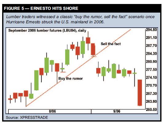
Compared to 2005, the 2006 Atlantic hurricane season turned out to be mild, with only nine named storms and five that reached hurricane strength. Hurricane Ernesto occurred at roughly the same time as Katrina the previous year, so let’s compare the lumber market’s reaction to Ernesto and Katrina. The storm that became Ernesto was a tropical depression on Aug. 24, 2006, as it moved just north of Grenada. September lumber was in a minor uptrend at the time, and choppy trade allowed for a moderate price rally. The following day, Aug. 25, Ernesto was upgraded to tropical storm status as it hovered south of Puerto Rico, and lumber futures staged a sharp rally, even briefly touching the $10 limit in the day’s session. The market continued to drift moderately higher for the next several sessions and made another sharp move higher on Aug. 30, when Ernesto made landfall near Plantation Key, Fla. in the early morning. Ernesto gained strength on Aug. 31 and lumber prices hit their peak of the move that day, as the storm headed up the east coast towards North Carolina. On Sept. 1, Ernesto moved ashore at Oak Island, N.C., and then moved across the state, where it weakened into a tropical depression. Lumber prices also weakened that day, closing near the lows of the day, which sparked a wave of long liquidation selling on Tuesday after the Labor Day holiday. Prices gapped lower on the opening and capped any further rally attempts for the remainder of the contract, which went off the board just above the contract low (Figure 5).
The bottom line
From 2004 to 2006, 13 named hurricanes hit landfall in the U.S. To see if the old adage “buy the rumor, sell the fact” held true, we looked at the closing price for the nearby lumber futures contract (if it fell within the delivery month, the next contract was used) on the day the storm first officially became a hurricane (rumor) and compared that to the closing price on the day the storm made landfall in the U.S. (news). Three of the storms acquired hurricane strength on the same day they came ashore in the U.S., so they didn’t provide trading opportunities (Table 1). Of the remaining 10 storms, six produced gains and four produced losses. Overall, a trader who bought the rumor (the date the storm became a hurricane) and sold the fact (the storm reached landfall in the U.S.) produced a net gain of $14.30 per contract. However, in some extreme cases, as with Hurricane Katrina, a major hurricane can completely turn around the trend and keep prices supportive for months.